Mapping the MNS model onto Java implementation
Erhan Oztop, May 2002
erhan@atr.co.jp
Last update: 18 June 2002
Jump to .....
1. A general introduction
2. Program level description and thread implementation
logic
3. Class Relationships
4. File Formats
5. Code level documentation
6. Download tar.gz ball for
1. A general introduction
The implementation
of MNS follows a schema-based approach. However, the implementation of
each schema in general requires multiple number of source files (java classes).
Several java classes are required to set up the stage for the simulation
environment and schemas and thus are not directly map to the model components.
We first summarize the schemas and indicate how and in which java classes
they have been implemented. A detailed `programmers view' of the simulation
system is presented afterwards.
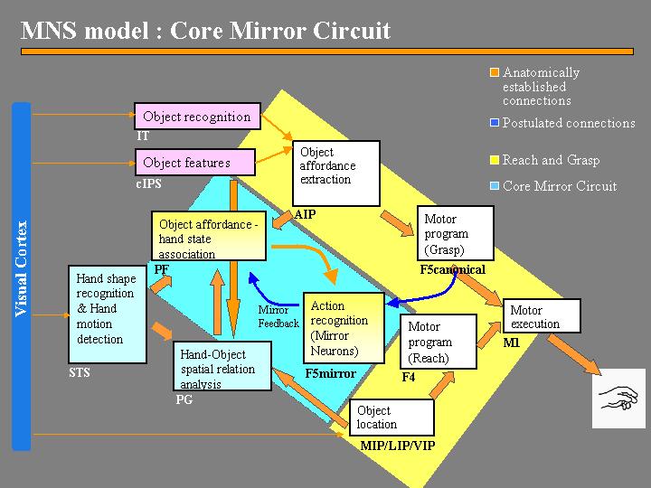
Figure 1. The MNS (Mirror Neuron System) model.The
grand schemas are illustrated as the following. The "Core Mirror Circuit"
schema is marked by the center blue box; The "Visual Analysis of Hand State"
schema is formed by STS and PG, and the "Reach and Grasp" schema is marked
by the yellow background.
The
overall system operates in two modes:
(i)
Prehension: In this mode, the system will perform grasping actions
according to the simulation parameters, such as the position and size of
the object. This mode is engaged in two steps. Clicking on VISREACH starts
the inverse kinematics solution process. After the solution has been obtained,
the grasp can be generated by clicking on REACH button.
(ii)
Action recognition: In this mode, the system engages the MNS model
embedded in the simulation system. To engage the MNS in recognition, first
a grasp action must be solved using VISREACH. Then clicking on RECOGNIZE
button will instantiate the MNS model and run the model as the grasp action
is taking place (the RECOGNIZE button will initiate the grasp action recently
solved).
A simplified
version of the system is provided online at http://java.usc.edu/~erhan/sim6.1/
that let users generate grasping actions (i.e. use the Reach and Grasp
schema) and query the grasp for action recognition (i.e. use the Core Mirror
Circuit schema)
1.1 The Three Grand Schemas
The schemas
shown in Figure 1, are encapsulated into the three "grand schemas" as shown
in Figure 2(a). The Reach and Grasp schema and the Core Mirror Circuit
schema are entirely contained in the simulation system. The video input
related functions of the Visual Analysis of Hand State are implemented
offline outside the simulation system. The class ImageProcess.java
implements the visual processing and feature extraction steps.
Figure 2.(a) For purposes of
simulation, the schemas of the MNS model (Figure 1) are grouped under three
"grand schemas" for Visual Analysis of Hand State, Reach and Grasp, Core
Mirror Circuit. (b) For detailed analysis of the Core Mirror Circuit, we
dispense with simulation of the other two grand schemas and use other computational
means to provide the three key inputs to this grand schema.
1.1.1
Grand Schema 1: Reach and Grasp
The simulator
lets us move from the representation of the shape and position of a (virtual)
3D object and the initial position of the (virtual) arm and hand to a trajectory
that successfully results in simulated grasping of the object. In other
words the simulator plans a grasp and reach trajectory and executes it
in a simulated 3D world. During a typical reach to grasp movement, the
hand will follow a `bell-shaped' velocity profile (a single peaked velocity
curve). The kinematics of the aperture between fingers used for grasping
also exhibits typical characteristics. The aperture will first reach a
maximum value that is larger than the aperture required for grasping the
object and then as the hand approaches to the target the hand encloses
to match the actual required aperture for the object. The simulator captures
the qualitative aspects of the typical reach and grasp actions, namely
that the velocity profiles have single peaks and that the hand aperture
has a maximum value which is larger than the object size. A grasp is planned
by first setting the operational space constraints (e.g., points of contact
of fingers on the object) and then finding the arm-hand configuration to
fulfill the constraints. The latter is the inverse kinematics problem.
The simulator solves the inverse kinematics problem by simulated gradient
descent with noise added to the gradient. Once the hand-arm configuration
is determined for a grasp action, then the trajectory is generated by warping
time using a cubic spline. The parameters of the spline are fixed and determined
empirically to satisfy aperture and velocity profile requirements. Within
the simulator, it is possible to adjust the target identity; position and
size manually using a GUI or automatically by the simulator as, for example,
in training set generation.The Grand Schema 1 is composed of the following
schemas:
Object
Features schema:The output of this schema
providesa coarse coding of geometrical features
of the observed object. In the simulation the object features are not represented
explicitly, instead the `right' object feature is directly encoded in the
Object-Affordance Extraction schema.
Object
Affordance Extraction schema :This schema
transforms its input, the coarse coding of geometrical features of the
observed object provided by the Object features schema, into a coarse
coding for each affordance of the observed object.
The transformation is not implemented instead this schema is taken as 10-unit
extension of the hand-state input and the representation is formed algorithmically
(i.e. no feature extraction). The current implementation encodes only the
size of the object. Note that there are different implementations where
the explicit object affordance is disabled. The class HandBP.java
performs the 10-unit coding for recognition.
Object
Location schema:The output of this schema provides, in some body-centered
coordinate frame, the location of the center of the opposition axis for
the chosen affordance of the observed object. This information is contained
in Graspable.java.
Motor
Program (Grasp) schema: The input to this schema is the object features
required for grasping. Conceptually this information is relayed via AIP.
In the implementation the class Graspable.java
contains the information about how to grasp an object. This output drives
the Action-recognition (Mirror neurons) schema as well as the hand
control functions of the Motor execution schema
Motor
Program (Reach) schema :The input is the
position coded by the Object location schema, while the output is
the motor command required to transport the arm to bring the hand to the
indicated location. This drives the arm control functions of the Motor
execution schema.
The
Motor Execution schema determines the course of movements via activity
in primary motor cortex M1 and "lower" regions. In the implementation the
reach and grasp configuration is used to generate and execute a grasping
action. This function is implemented in Object3d.java
via the thread execution system.
1.1.2 Grand Schema 2:Visual Analysis of Hand State
Visual
Analysis of Hand State Schema is a non-neurophysiological implementation
of a visual analysis system to validate the extraction of hand parameters
from a view of a hand, by recovering the configuration of a model of the
hand being seen. The hand model is a three dimensional 14 degrees of freedom
(DOF) kinematic model, with a 3-DOF joint for the wrist, two 1-DOF joints
for each of the four fingers, and finally a 1-DOF joint for the metacarpophalangeal
joint, and a 2-DOF joint for the carpometacarpal joint of the thumb. Note
the distinction between "hand configuration" which gives the joint angles
of the hand considered in isolation, and the "hand state" which comprises
7 parameters relevant to assessing the motion and preshaping of the hand
relative to an object. Thus the hand configuration provides some, but not
all, of the data needed to compute the hand state. To lighten the load
of building a visual system to recognize hand features, we mark the wrist
and the articulation points of the hand with colors. We then use this color-coding
to help recognize key portions of the hand and use this result to initiate
a process of model matching. Thus, the first step of the vision problem
is color segmentation, after which the three-dimensional hand shape is
recovered.
Color
Segmentation and Feature Extraction
Color segmentation
is implemented using, split-and-merge method that works by recursively
splitting the image into smaller pieces until some homogeneity criterion
is satisfied as a basis for reaggregation into regions. In our case, the
criterion is having similar color throughout a region. However, RGB (Red-Green-Blue)
and HSV (Hue-Saturation-Value) were not satisfactory for our purposes due
to shading and the inherent low quality of the video input. Therefore,
we designed an adaptive system that can learn the best color space (color-expert).
The system is a (one hidden-layer) feed-forward network with sigmoidal
activation function. The network is given around 100 training samples manually
using the GUI implemented in ImageProcess.java
each of which is a vector of ((R, G, B), perceived color code) values.
The training is done only at the beginning of a session to learn the colors
used on the particular hand. Then the network is fixed as the hand is viewed
in a variety of poses. The output of the algorithm is then converted into
a feature vector with a corresponding confidence vector giving a confidence
level for each component in the feature vector. Each finger is marked with
two patches of the same color (see Figure 3). Sometimes it may not be possible
to determine which patch corresponds to the fingertip and which to the
knuckle. In those cases the confidence value is set to 0.5. If a color
is not found (e.g., the patch may be obscured), a zero value is given for
the confidence. If a unique color is found without any ambiguity then the
confidence value is set to 1. The segmented centers of regions (color markers)
are taken as the approximate articulation point positions. Toconvert the
absolute color centers into a feature vector we simply subtract the wrist
position from all the centers found and put the resulting relative (x,y)
coordinate into the feature vector (but the wrist is excluded from the
feature vector as the positions are specified with respect to the wrist
position). The image processing routines are implemented in ImageProcess.java.
The training of the color expert is also performed within this class. The
learning engine resides in BP.java. The output
of ImageProcess is feature file to be used with the 3D model matching routines.
3D Hand Model Matching
Our
model matching algorithm uses the feature vector generated by the segmentation
system to attain a hand configuration and pose that would result in a feature
vector as close as possible to the input feature vector (Figure 3).
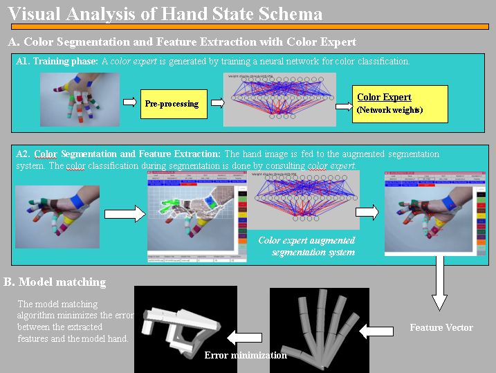
Figure 3. Illustration of the model matching
system. Left: markers located by feature extraction schema. Middle and
Right: initial and final stages of model matching. After matching is performed
a number of parameters for the Hand configuration are extracted from the
matched 3D model.
The
matching algorithm is based on minimization of the distance between the
input feature and model feature vector, where the distance is a function
of the two vectors and the confidence vector generated by segmentation
system. Distance minimization is realized by hill climbing in feature space.
The distance between two feature vectors F and G is computed
as follows:
where
subscripting denotes components and Cf, Cg
denotes the confidence vectors associated with F and G. The
model matching code is implemented by Match.java,
Feature.java.
When
we simulate the Core Mirror Circuit (Grand Schema 3) we will in general
not use this implementation of Visual Analysis of Hand State but instead,
to simplify computation, we will use synthetic output generated by the
reach/grasp simulator to emulate the values that could be extracted with
this visual system. Specifically, we use the hand/grasp simulator to produce
both (i) the visual appearance of such a movement for our inspection (Figure
4 Left), and (ii) the hand state trajectory associated with the movement
(Figure 4 Right). Especially, for training we need to generate and process
too many grasp actions, which makes it impractical to use the visual processing
system without special hardware as the computational time requirement is
too high.The Grand Schema 2 is composed of the schemas:
The Hand
Shape Recognition schema takes as input a view of a hand, and its output
is a specification of the hand shape, which thus forms some of the components
of the hand state. In the current implementation these are a(t), o
3 (t) and o 4 (t). Note also that we implicitly assume
that the schema includes a validity check to verify that the scene does
contain a hand . This function is implemented
offline. The color segmentation and color expert training are performed
with ImageProcess.java. The 3D hand
matching is contained in the simulation system but requires a hand-only
kinematics chain model of the hand. Since the many of our simulations use
the emulated hand state bypassing the visual analysis of a real video sequence.
We will not describe the methods making up 3d hand matching in detail.
The Hand
Motion Detection schema takes as input a sequence of views of
a hand and returns as output the wrist velocity, supplying the v(t) component
of the hand state. This supplied via the Reach and Grasp simulator substituting
the actual video processing.
The
Hand-Object
spatial relation analysis schemareceives object-related signals from
the Object features schema, as well as input from the
Object
Location, Hand shape recognition and Hand motion detection
schemas. Its output is a set of vectors relating the current hand preshape
to a selected affordance of the object. The schema computes such parameters
as the distance of the object to the hand, and the disparity between the
opposition axes of the object and the hand. Thus the hand state components
o 1(t), o 2 (t), and d(t) are supplied by this schema.
In the implementation the hand-object relation is computed algorithmically
and the resultant vector (hand state) is encoded in the output, which is
relayed to the Object affordance-hand state association
schema.
In turn Object affordance-hand state association schema drives the
F5 mirror neurons whose output is a signal expressing confidence that the
observed trajectory will extrapolate to match the observed target object
using the grasp encoded by that mirror neuron.
To recap,
in the implementation Reach and Grasp schema is used to (1) plan and execute
reach and grasp (render a graphical view of the hand and the object during
grasping) (2) Emulate the Visual Analysis of Hand State schema and produce
the Hand State that is used by the Core Mirror Circuit.
1.1.3 Grand Schema 3: Core Mirror Circuit
As diagrammed
in Figure 2(b), the analysis of the Core Mirror Circuit does not require
simulation of Visual Analysis of Hand State and of Reach and Grasp so long
as we ensure that it receives the appropriate inputs. Thus, we supply the
object affordance and grasp command directly to the network at each trial.
(Actually, we conduct experiments to compare performance with and without
an explicit input which codes object affordance.). Rather than provide
visual input to the Visual Analysis of Hand State schema and have it compute
the hand state input to the Core Mirror Circuit, we use the reach and grasp
simulator to simulate the performance of the observed primate -
and from this simulation we extract both a graphical display of the arm
and hand movement that would be seen by the observing monkey, as
well as the hand state trajectory that would be generated in his brain.
We thus use the time-varying hand state trajectory generated in this way
to provide the input to the model of the Core Mirror Circuit of the observing
monkey without having to simultaneously model his Visual Analysis of Hand
State. Thus, we have implemented the Core Mirror Circuit in terms of neural
networks using as input the synthetic data on hand state that we gather
from our reach and grasp simulator.
Neural Network Implementation
For supervised
learning that takes place in the Core Mirror Circuit, we used a feed-forward
neural network with one hidden layer. We can here identify the parts of
the neural network as Figure 1 schemas in a one-to-one fashion. The hidden
layer of the model neural network corresponds to the Object affordance-hand
state association schema, while the output layer of the network corresponds
to the Action recognition schema (i.e., we identify the output neurons
with the F5 mirror neurons). In the following formulation, MR
(mirror response) represents the output of the Action recognition schema;
MP
(motor program) denotes the target of the network (copy of the output of
Motor
Program (Grasp) schema ). X denotes the input
vector applied to the network, which is the transformed Hand State tajectory
(and the object affordance). The transformation applied is described in
the next subsection. The learning algorithm used is implemented in the
class HandBP.java.
Temporal
to Spatial Transformation
The input at any time represented the entire input from
the start of the action until the present time t. To form the input vector,
each of the seven components of the hand state trajectory to time t is
fitted by a cubic spline, and the splines are then sampled at 30 uniformly
spaced intervals (see Spline.java). The hand
state input is then a vector with 210 components (220 for the explicit
object affordance coding simulations): 30 samples from the time-scaled
spline fitted to the 7 components of the hand-state time series. Note then
that no matter what fraction t is of the total time T of the entire trajectory,
the input to the network at time t comprises 30 samples of the hand-state
uniformly distributed over the interval [0, t]. Thus the sampling is less
densely distributed across the trajectory-to-date as t increases from 0
to T. The class Spline.java provides routines
to collect vector of parameters and then return a spline representation
out of the collected data. The scaling operation is also implemented in
this class.
The
Neural Network Training
The training set was constructed by making the simulator
perform various grasps in the following way.
(i) The
objects used were a cube of changing size (scaled randomly by 0.5 -1.5),
a disk (approximated as a thin prism), a ball (approximated as a dodecahedron)
again scaled randomly by a number between 0.75 and 1.5. In this particular
trial, we did not change the disk size. In the training set formation,
a certain object always received a certain grasp (unlike the testing case).
(ii) The
target locations were chosen form the surface patches of a sphere centered
on the shoulder joint. The patch is defined by bounding meridian and parallel
lines. The extent of the meridian and parallel lines was from -45°
to 45°. The step chosen was 15°. Thus the simulator made 7x7 =
49 grasps per object. The unsuccessful grasp attempts were discarded from
the training set. For each successful grasp, two negative examples were
added to the training set in the following way. The inputs (group of 30)
for each parameter are randomly shuffled. In this way, the network was
forced to learn the order of activity within a group rather than learning
the averages of the inputs (note that the shuffling does not change mean
and variance). The second negative pattern was used to stress that the
distance to target was important. The target location was perturbed and
the grasp was repeated (to the original target position). Another modification
to the training was to introduce a random input pattern (totally random;
no shuffling) on the fly during training and ask the network to produce
zero output for those patterns. The learning engine is implemented
in HandBP.java where as the training data generation
explained above is performed by the generateData method of HV.java.
The class Learn.java is used in collecting
hand state data for both training data generation and recognition.The Grand
Schema 3 is composed of the schemas:
The Action
Recognition schema corresponds to the mirror neurons of area F5 and
receives two inputs in our model. One is the motor program selected by
the Motor program schema; the other comes from the Object affordance-hand
state association schema. This schema works in two modes: learning
and recognition. When a self-executed grasp is taking place the schema
is in learning mode and the association between the observed hand-state
(Object affordance-hand state association schema) and the
motor program (Motor program schema) is learned. While in recognition
mode, the motor program input is not active and the schema acts as a recognition
circuit.
The
Object affordance-hand state association schema combines all the hand
related information as well as the object information available. Thus the
inputs to the schema are from Hand shape recognition (components
a(t), o3(t), o4 (t)), Hand motion detection
(component v(t)), Hand-Object spatial relation analysis (o
1 (t), o2 (t), d(t)) and from Object affordance extraction
schemas. As will be explained below, the schema needs a learning signal
(mirror feedback). This signal is relayed by the Action recognition
schema and, is basically, a copy of the motor program passed to the Action
recognition schema itself. The output of this schema is a distributed
representation of the object and hand state match which is shaped by the
learning process. The idea is to match the object and the hand state as
the action progresses during a specific observed reach and grasp. In the
current implementation, time is unfolded into a spatial representation
of "the trajectory until now" at the input of the Object affordance-hand
state association schema, and the Action recognition schema decodes
the distributed representation to form the mirror response.
In short,
the schema has two operating modes. First is the learning mode where the
schema tries to adjust its efferent and afferent weights to ensure the
right activity in the Action recognition schema. The second mode
is the forward mode where it maps the hand state and the object affordance
into a distributed representation to be used by the Action recognition
schema.
2. Program level description and thread implementation
logic
The simulator
environment is designed such as new behavior or tasks required it can be
added to the system. For example a click on the VISREACH button initiates
a grasp planning task; a click on REACH button initiates an other task
namely executing the recently planned task. Some tasks can run in parallel.
A click on YROTATE button will put the camera into an orbit around the
Y-axis. While the camera is rotating other tasks can be initiated (e.g.
VISREACH). In what follows I will explain how to add a new task by going
through the VISREACH mechanism in detail.
The GUI
of the simulation environment is implemented in HV. Every event in the
simulator starts from a user action. The events are initially handled by
HV.java.
Thus
the entry points of tasks reside in HV.java
To run
the system type:
java
HV
OR
java
HV [.seg file [sidec radius [feat file?]]]
The .seg
file defines the arm object to be loaded as a Segment class (see Segment.java).
Each object can have many segments possible but currently only single segment
is used. The parameters sidec and radius define the cylinder drawn around
the skeleton. The feat file is the feature file that is extracted by ImageProcess.java
and used for 3D model matching.
The
user starts a grasp planning by hitting VISREACH, which triggers the system
to start solving the inverse kinematics problem involved. When HV is notified
that the user hit VISREACH, the method toggleReach() (in HV.java)
is called. This method may initiate various type of grasps as indicated
by its parameter. Or it can initiate a `natural' grasp corresponding to
the current object The default affordances and grasping types for objects
are defined in Graspable.java. The natural()
method of Graspable will be called if a natural grasp is requested. For
any object any grasp can be enforced by the user via the GRASPTYPE button.
When
toggleReach() is called if there was an active reach task (checked by Hand.reachActive())
the reach/grasp is terminated by Hand.kill_ifActive(). Let's assume that
we made a natural reach/grasp plan and there was no active task. Natural
grasp choice directs the program flow to precision, power etc methods in
Graspable. Currently each Graspable affords one grasp type (unless manually
changed by the user). Let's assume the grasp to be executed is precision.
Then the method precision() in Graspable.java
will be called. In general, the grasp planning is done by determining some
targets on the object for the hand and trying to achieve a specified contact.
The tIndex[] array is used to hold segment pointers to indicate the parts
of the hand that are used in targeting. The variable target holds the actual
values (numbers) to be achieved. After the kinematics goals are set the
control returns to HV.togglereach() and Hand.doReach(object, s) is called.
Hand.java
is a superclas s of Object3d.java
and infact doReach is in Object3d.java
(bad programming). The method doReach(s) is the control center for actions.
When the control reaches doReach(), the program execution is multiplexed
according to the parameter passed (s).
-
If s='visual' then fireVisualSearch() is called.
-
If s='execute' then fireExecution() is called.
-
If s='record' then firstly Learn.PrepareforPattern() is called
to setup for data collection (for training data generation) and recordit
is set to true indicating that the generated hand state trajectory data
will be stored. Finally fireExecution() is called to create the reach thread.
-
If s='recognize' then firstly Learn.prepareforPattern() is
called to setup for recognition task (for mirror response) and the
variable recognize is set to true indicating that the formed hand state
trajectory data will be sent to Core Mirror Circuit for a response. Finally
fireExecution() is called to create the reach thread.
Let's
look at fireVisualSearch(). The method performs some initialization and
creates the reach thread. A hook to object to be grasped is provided for
execution of possible actions before the reach (obj.beforeAction()). The
reach thread knows the mode it is in by reading the search_mode variable.
Since this is VisualSearch, we set search_mode to VISUAL_SEARCH. Visual
search refers to the solution of the inverse kinematics problem for the
grasp without hiding the steps from the user. The thread is created using:
activeReachThread=
createReachThread("");
The
value returned from createReachThread is returned by fireVisualSearch().
The method createReachThread() starts the actual Java thread and does some
initialization and starts the execution of the thread. The Reach.java
class extends the Java supplied Thread class, which is pretty simple and
short. The Reach.java is started with its
start() method. After this, the control switches to the run() method (this
is performed by the Java run-time environment - run() is not called directly).
The run() method of Reach loops forever and invokes different methods according
to obj.search_mode. For example if it is obj.VISUAL_SEARCH then the corresponding
`tick' method in Object3d is called. (e.g. obj.tickVisual(this)). The `tick'
methods of Object3d.java perform a step
of a whole action and exit. Thus the functioning of the `tick' methods
rely on the repeated call from the created and started Reach thread. The
Reach thread also calls HV.cv.refreshDisplay() after the tick method is
called for redrawing what happened. The run() of the Reach thread loops
until the variable stopRequested is changed to true from somewhere outside,
indicating either a user abort, error, or completion of the task. For example
when the inverse kinematics is solved (i.e. Visual Search task completes),
tickVisual() will set stopRequested to true when the solution is found.
When the run() loop receives the stop request it performs some finalization
stuff including a call to finalizeReach(c) method in the Graspable.java
class.
3.The Class Relationships
The functionality
that is provided with the classes that make up the simulation environment
can be grouped as (1) support classes (2) 2D display and GUI (3) 3D engine
(4) Control classes and finally(5) MNS related classes. Unfortunately,
due to programming convenience (limited programming time or program efficiency)
some classes are involved in more than one function.
1.The
support classes are VA.java and Elib.java.
The former supplies matrix and vector algebra routines. The VA methods
are primarily used by the 3D engine classes. Elib.java
contains convenience methods that are usually short and simple such as
string manipulation and file I/O shortcuts.
2.The
2D drawing is handled by HVcanvas.java. The requests to refresh the display
is made to this class. Double buffering for a fine animation is also handled
in this class. HV.java is one of the multi function
classes and sets up the GUI and dispatches the user events.
3.Eye.java
contains methods for projecting the 3D environment to 2D view. The 3D environment
(objects) are kept and managed by the class Mars.java.
Some of the 3D rendering and object interaction operations are performed
within Object3d.java such as 3D solid rendering,
collision detection, inside/outside detection.
Figure 4. Some of the simulation
system components and their major function.
4.
Control classes are the programming constructs enforcing a certain style
of programming to achieve correct sequence of processing. For example,
the way the thread system (described in the previous section) set up requires
certain book keeping methods. Unfortunately, in terms of object orientation,
the code here is not well written. Virtually
HV.java
and
Object3d.java form the skeleton of
the control system. HV initiates a task, which eventually leads to a call
to
Object3d.java. Object3d sets up some
flags and parameters according to the request from HV. It eventually creates
a thread that calls back the appropriate methods in Object3d and in other
classes.
Figure 6. The major components of the simulation
system that makes up the Reach and Grasp and the Core Mirror Circuit schemas.
5.The
MNS routines are distributed over Segment.java,
Object3d.java,
Hand.java,
Learn.java
and BP.java.
Segment.java
keeps the kinematics of the arm and have routines to manipulate the arm/hand.
Thus it is part of the Reach and Grasp schema. It performs the forward
kinematics computation required by the 3D rendering routines. The forward
kinematics problem is the calculation of the position and orientation of
the links making up the arm/hand in 3D space given the geometry of the
hand/arm and the joint angles. The geometry of the arm/hand is specified
in .seg file which can read from Segment.java.
Hand.java
defines some hand related variables and contains methods specific to arm/hand
object such as computing the aperture.
Learn.java
and BP.java correspond to the MNS model's hand
state generation and the functioning of the core mirror circuit. Learn.java
can collect data and represent them as splines. During training set generation
Learn.java
collects data and writes them to the disk in a way that BP.java
can read it offline and used it in training. During recognition Learn.java
collects hand state data forms the input (spline fitting and normalization)
to BP.java and queries BP with the input.
4. File formats
The
segment (.seg) file format:
The hand/arm and the objects for grasping are defined
by segment files. The file must be ASCII text and must follow the convention
described below. I will use the actual arm/hand definition file to describe
the format:
#The
sharp (#)character indicates a comment. Empty lines are ignored.
#
The keywords are shown in red color.
# Eye is specifies the default Fz, F, and scale values
for projection. Usually fixed.
# The coordinate system is left-handed. +z axis goes
into the screen, +y axis is the vertical
# axis going upwards on the screen. +x axis is the horizontal
axis towards the right of the
# screen.
# Below setting gives a lens at 0,0,-9500 looking at
0,0,0 with mag=900
Eye
0 9500 900
#
The links (or segments or limbs) are defined hierarchically. The parents
of a link
# can be referenced with either ID or label
# Note that the base of the fingers are fixed joints!
Thus base+1 base+2
# are flexible joints.wrist is also flexible.
# Note that JointPos LimbPos JointAxis are index to Points
(starting from 1)
# ID must be greater than 0. A zero parent means null
parent.
# * jointAxis is actually is the cross product of the
limb with the value given
# under JointAxis.
#AxisType=0 (or jointaxis=(0,0,0) ) means fixed joint.
#AxisType=-1 means that the JointAxis given is not actually
the joint axis;
#to get the real joint axis a cross product of the axis
with
#(jointpos-limbpos) is required (this is done by the
file loader)..
#AxisType=1 means the JointAxis field IS actually the
joint axis.
# Limbs starts the definition of the links of the kinematics
chain
Limbs
#
The first column is a user-defined label. In this case, it defines the
first link the
# (upper arm) and the first joint. Next three numbers
(JointPos) is the position of the joint
# as (x,y,z). Next three (LimbPos) define the position
of the end of the link. The next three
# (JointAxis) define the rotation axis of the limb (see
above for special values). The next
# number (Jtype) defines thee joint type (see above for
special values). The last value
# (Parent) indicates which link this link is connected
to.
# Note that in the below BASE just sets the shoulder
position but does not define a joint.
# The length of the link is 0 (JointPos and LimbPos are
the same)
#LABEL JointPos
LimbPos JointAxis
JType Parent
BASE 0 0 -750
0 0 -750 0 0 0
0 -1
# Within the optional section of Points-EndPoints some 3D points can
be defined for later
# referencing in the Planes section. The idea is to enable of covering
the limb with user
# defined planes for visualization reasons.
Points
300 700 -350
400 800 -350
400 800 50
300 700 50
-1200 -1700 -1200
-1200 -1700 1200
1200 -1700 1200
1200 -1700 -1200
EndPoints
# Now we define the actual joints. J1, J2, J3 implements the 3DOF of
the shoulder. Note the<>
# labels in the last column where the hierarchy is set.
#LABEL JointPos
LimbPos JointAxis
JType Parent
J1
0 0 0 0 0 0
1 0 0 1
BASE
J2
0 0 1 0 0 0
0 0 -1 1
J1
J3
0 0 1 0
-800 0 -1 0
1 J2
J4
0 0 1 0 0 0
1 0 0 1
J3
WRISTz 1 0 0
0 0 700 0 0
1 1
J4
# Other links are specified similarly. Note that the link length information
is implied
# by the joint position and limb position values.
WRISTy 0.00 0.00 0.00
0.00 0.00 0.00 00 01 00
01 WRISTz
WRISTx 0.00 0.00 0.00
0.00 0.00 0.00 01 00 00
01 WRISTy
PINKY 0.00 0.00
0.00 83.00 0 144.00 00
-01 00 -1 WRISTx
PINKY1 0.00 0.00 0.00
32.00 0 45.00 00 -01 00 -1 PINKY
PINKY2 0.00 0.00 0.00
39.00 0 50.00 00 -01 00 -1 PINKY1
RING 0.00 0.00
0.00 45.00 0 152.00 00
-01 00 -1 WRISTx
RING1 0.00 0.00
0.00 22.00 0 91.00
00 -01 00 -1 RING
RING2 0.00 0.00
0.00 30.00 0 79.00
00 -01 00 -1 RING1
MIDDLE 0.00 0.00 0.00
0.00 0 159.00 00 -01 00 -1 WRISTx
MIDDLE1 0.00 0.00 0.00
5.00 0 108.00 00 -01 00 -1 MIDDLE
MIDDLE2 0.00 0.00 0.00
11.00 0 89.00 00 -01 00 -1 MIDDLE1
INDEX -12.00 0.00 0.00
-55.00 0 156.00 00 -01 00 -1 WRISTx
Points
0 5 0
EndPoints
INDEX1 0.00 0.00 0.00
-16.00 0 87.00 00 -01 00 -1 INDEX
Points
0 5 0
EndPoints
INDEX2 0.00 0.00 0.00
-9.00 0 76.00 00 -01 00 -1 INDEX1
THUMB -35.00 0.0 -5.00
-35.00 0 10.00 00 0 1 01 WRISTx
THUMBin 0.00 0.00 0.00
-98.00 0 0.00 00 01 00 01 THUMB
THUMB2 0.00 0.00 0.00
-90.00 0 0.00 00 1 0 01
THUMBin
Points
0 0 0
EndPoints
THUMB3 0.00 0.00 0.00
-50.00 0 0.00 00 1 0 01
THUMB2
# Planes section draws planes by referencing the Points defined before.
# For example the first line after the Planes keyword below draws a
triangle between the
# thumb and index for a more pleasent look.
Planes
INDEX 0 INDEX1 0 THUMB2 0 INDEX 0
The
BP weight (trained network specification) file format:
The BP saves the trained network parameters in a weight
file. The weight file then can be used for recognition within the simulation
system. The format of the weight file is as follows.
# This file
specfies the network size and the weight values
# Network
sizes exclude the clamped 1's for input and hidden layer
# So the
weight matrices has one more column for the clamped unit.
# Note: To
train the network you need to load a pattern file
# Note:
One can not specify learning parameters from this file
# Note:
If it is desired to continue a learning session that has been partially
learned and
# saved
as a weight file,the user should use Make Network from Weight followed
by Load Pattern
# and then
continue training.
# First matrix
is the input(x)->hidden(y) weights(w)
# Second
matrix is the hidden(y)->output(z) weights(W)
# The network
computes sgn(W.sgn(w.x)) where sgn(t)=1/(1+exp(-t))
#
number of output units
outputdim
12
#
number of hidden units
hiddendim
15
#
number of input units
inputdim
3
#
The rest of the file must contain two matrices: First one is the input
to hidden unit weights
# and must
be of size (hiddendim+1)x(inputdim+1). The second matrix specifies hiddendim
to output
# weights
and must be of size (hiddendim+1)x(outputdim. The rest of the file also
may contain
# comments
(# lines) or spaces.
#
NOTE: this is a sample weight data and is not related to the hand state
trajectory.
#
input -> hidden weights w[16][4]
10.422786741951482
16.73426199413754 -7.466200723034477 -12.787040187558674
16.499510172456855
4.90012092736305 -28.022539006345056 -0.9427094535978825
-17.6886996507937
-5.020396213129124 18.63473513981201 -7.419837675439184
16.897785745600636
-5.413514084920573 15.380053975037333 -13.907545708819363
27.56417841807994
-12.780044737056045 1.615048155203243 -13.168763882615979
-33.44896959556014
3.1760776694926887 9.262262475538996 -1.2742324888058414
-21.407252177972133
22.582425819119617 -4.87055954571949 -3.24997130962201
5.135055034713992
29.89695887312792 -2.4656355197730124 -6.379078899867055
29.580412926937058
-26.6922637332009 9.680411652169438 -5.554100916880081
4.1819164726456295
-1.8921208436907047 -9.430850780797586 -2.2017384680840513
30.942311345861352
-26.665355203358835 -4.662884666887864 -0.7986902810193839
6.465607424246219
23.93106115639326 -25.846052510815646 -3.5599676455190195
-11.225871018176264
-17.717022914584547 26.964441701700064 -4.129314058546056
6.976397172393547
-15.700935596088472 -0.2986705879703097 -0.6253219045074162
6.293018483956897
-0.13658205945008037 19.87570954904005 -9.101282738417348
0.013026976553848647
0.02055113570277364 0.003055647740781431 -0.007700128556778718
# hidden
-> output weights W[12][16]:
-14.194373045068529
-3.531086734189389 -6.70011522925556 -2.1080285956872906 -7.072482901221429
-11.317620850123792 13.646290412167643 -0.35448280286673767 -15.30901422135202
-2.412323898046175 -4.719923931253326 -19.190783152544284 -5.1458711660356
-3.0707297172778114 6.031155234692427 -9.708743931800873
-12.95428038244905
-2.512048414824848 -4.108109331897354 -10.131199015152907 12.869434870837223
-2.557542014875756 -4.9747969991352665 8.656391901314256 3.602040419669517
-5.228865715695639 -6.047442278840204 7.354443855483113 -5.098154500418354
0.810851488745853 -10.84546263647792 -15.049137183991494
-1.3208256591716374
-2.8748717603584057 -3.6290118185950275 -6.94193876011284 -6.16976662364653
-12.708403205187519 -7.3627651345216885 -15.294504309232858 11.93232757072578
-1.3851944125883646 -17.53039217390351 -2.4495412287481106 4.309977728613909
-5.411186368310457 2.0137278126699525 -2.2959194719567493
-2.018364375291581
-7.671290219312747 -4.986309494153618 -4.67928127438167 -2.07043036773269
0.9922638329891751 11.294378718570114 -3.5535147898191815 -7.027124136383734
-1.4352053566750311 -4.755562620102474 -13.047279080208025 -9.449719682579724
-4.056473356555448 -11.153474554232359 -1.4980636589887397
-2.164923119711553
-13.618487180407401 -3.619415633364873 -4.241557476565329 0.03612462718988775
-3.470311133518886 -3.9288286929908116 -12.220065240378437 3.5439207283817673
-2.889494610019677 6.814436125254603 -10.00700473378317 -12.965733102711402
8.558465674310087 -1.0867560866291053 -9.082973687447884
-3.2229012661859526
-3.1238896844408623 10.149725270407197 -12.537562128516486 -3.921951764568255
-2.6442871778320765 -12.076693344525038 -13.343435559812383 -8.723901021543902
-2.893166398333897 -7.352508110442664 -4.120317950656725 4.691342404427895
-5.3562148926079605 3.812237132555929 -7.384676482517599
10.656960742098745
-0.030958259070857554 -2.8275106720610657 0.13977793306768035 -9.47648839039812
-2.191330866593963 -13.128322774913409 -1.7899503816001672 -11.694390627542345
-2.1297029158879144 11.314607962793469 -2.4885181754719183 -3.399231331208309
-5.917827068358364 -0.9473786831822668 -11.03501447719245
-1.633367930356288
0.1703034598094734 -0.8775529129215793 -5.347910958554222 -5.105415617019582
-4.7114174488156735 -4.535867458702889 -9.290743939562235 -17.13750406562645
-1.1262823670832158 11.088705894099176 -6.6057143939286735 -6.391820318627141
-4.075227376593448 -5.205309263962132 -1.672760935870957